Detailed web-based 3D rendering of mining spatial data
This post explores the technology stack of rendering 3D data through a web browser, and the techniques used to make a responsive viewer. The project can be found here and there is a (very) rudimentary web app here. Note that the project is in the extremely early prototyping phase, exploring and validating techniques to get spatial data rendered on the web. The goal is to provide a practical application for others to build atop of.
Challenges
3D rendering of mining spatial data presents challenges that routinely abuts against hardware constraints and loop performance. It is not uncommon to see spatial data in the hundred megabyte to gigabyte range, and the ease at which technologies such as LiDAR can create extreme dataset sizes makes source data a burden to work with. This burden generally trickles down to how the data will be used. A topology scan might not need centimetre level of detail, but loading and simplifying this takes time. The amount of detail needed also changes in scope, but carrying around multiple variants of a file at differing simplification levels is difficult. Further to this, when finer detail is required, we have to go back to the larger and larger spatial files, which can overwhelm a rendering system just by the sheer amount of data. Typically the whole dataset is not needed at finer detail, but unless you carry around subsets of the areas, there is no way to avoid loading the whole file in.
Level of detail and tiling
Mapping software and the game industry both have techniques for dealing with similar problems. Game rendering engines typically use level of detail (LOD) as a way to reduce rendering burden. The technique provides multiple variants of the same object with differing levels of detail (duh!), so when an object is distant in the viewport (screen coverage is typically used as a metric), a low LOD object is rendered, whereas when an object is close, a high LOD object is rendered. It is important to note that LODs in games are usually stored in memory. The bottleneck is generally in rendering a scene quickly to achieve high frame rates, rather than rendering numerous triangles.
Mapping software uses the technique of tiling to avoid loading excessive amounts of data into the renderer. (Side note, they also use LODs, usually in a quadtree structure.) Since maps are (generally) 2D, it is trivial to render only the tiles which intersect with the viewport. Mapping software usually streams the tiles, from disk or server, which allows for a very small memory footprint. Indeed, loading a complete set of maps into memory would likely be infeasible.
Both these techniques could be employed for rendering mining spatial datasets, being particularly applicable to topological scans or data that is stratigraphically expansive. It is worth noting that LOD data would not be able to be stored in memory (basically we would be back to square one with hardware limits as discussed in Challenges). We also generally use orthographic projection in CAD work rather than perspective projection common in games. This has impacts for LODs, since distance along the depth axis does not 'vanish'.
Tech Stack
Whilst tiling and LOD techniques could be employed with any renderer, they would be particularly useful for rendering on lower performance systems. We have also seen a massive improvement in browser based 3D rendering, with the imminent release of WGPU, rendering through a browser will be the future. I also wanted to try using WASM with Rust, since I already have a geom library which has many tried and tested spatial algorithms geared towards the mining industry and I realllly did not want to implement them in Typescript.
For the 3D rendering engine, I decided to use BabylonJS. I have used it previously (with rrrehab) so I am familiar with many of its quirks, and implementing an engine would detract from the experiment. I have tried to keep the implementation independent of the engine so we are not tied to a backend.
The front-end I have used familiar Elm, but it is very rudimentary and mostly there to get things rolling. The viewer itself is buildable as a library and independent of the UI.
Another concern is avoiding blocking the UI thread. Processing mining data is slow, even with smart algorithms, the amount of data to process will consume noticeable time. It was imperative that this processing can be done off the UI thread, and for that we have to use WebWorkers.
And finally, as I indicated previously, this data cannot be kept in memory, so we need a mechanism to persist data. I settled on using another web API, IndexedDB, although I have not been thrilled with its characteristics. There is a proposed Filesystem API which could be leveraged in the future, for now IndexedDB is sufficient to store the blobs of bytes.
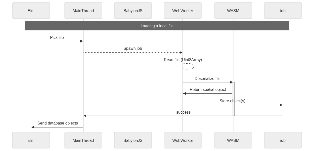
Each of these items present some interesting challenges around memory management and memory boundaries. As an example, the below chart shows the interactions of loading a local file.
Loading and preprocessing a surface
We'll focus on rendering a surface. Surfaces are made up of triangles in a triangle mesh. Surfaces can be considered 2.5 dimensional, they do not consist of overlapping triangles in plan view. There is nothing stopping a triangle mesh from having this property, but we'll assume that it holds true such that we can leverage sampling to obtain LODs. Currently, only loading in Vulcan 00t triangle mesh files is supported, other file formats are not the priority to evaluate the techniques.
Loading a local file consists of picking the file, reading the file into a byte buffer, and finally deserializing it into a triangle mesh. We want to offload this process onto a thread, and luckily a JS File can be transferred to a WebWorker thread. WebWorkers are interesting. They run code which is completely run in a separate scope, and in the wonderful world of JS means the code to run a WebWorker is separately fetched and loaded! There are some helper libraries, of which I am using threads-es, but because of the delineation, code to be run in a web worker is generally best kept as its own entry point. Below is the worker function which reads and parses the Vulcan file.
// worker.ts
// this defines my WebWorker API; functions to run on separate thread
const api = {
    read_load_and_store_from_spatial_file,
    preprocess_spatial_object,
    build_vertex_data
};

export type WorkerApi = typeof api;

exposeApi(api); // used for threads-es

// we can pass through a File just fine
async function read_load_and_store_from_spatial_file(db_name: string, file: File) {
    // but returning a TriangleMeshSurface will fail!
    let obj = await local_loader.parse_file(file);

    let db = await Store.connect(db_name);
    // so we store the object in the same function 😢
    await db.store_object(obj.name ?? 'new-object', obj.obj);
}
Notice that we do not split the two activities of parsing and storing the object into two functions. This is a major limitation of WebWorkers, because they communicate by message passing, one must be careful about where objects live. We run into two problems:
- Messages are deeply cloned, so passing through a massive mesh is a no-no,
- Classes coming from WASM are just pointers (more on that later), and cannot be passed across the boundary.
There is an exception (Transferable objects) which can pass things like ArrayBuffer through and effectively 'move' the value without cloning. I utilise this when generating the vertex data for rendering representations.
So we are forbidden from passing a TriangleMeshSurface across the WebWorker boundary, and even if it was not forbidden, we still would not want to be doing so because it is expensive. Luckily, the IndexedDB API is available in WebWorkers, and we can open up the same database and write to it. It is a bit annoying, since any DB interactions will need the database name passed through (and that is not static since we might want to run multiple DBs), but it does work and it is all happening off the UI thread.
Once we have a structured triangle mesh stored in the DB, we can proceed to preprocess it into various representations of tiles+LODs. This step on a high level is simple, get the object that was just stored from the store (invoked in a WebWorker), and then proceed to generate the representations, storing each representation as it goes. There are a few minor optimisations such as working out the tiles that will be generated by the mesh, and generating a simple bucketing hash to increase locality of sampling.
async function preprocess_spatial_object(db_name: string, objkey: string) {
    const db = await Store.connect(db_name);
    const mesh = await db.get_object(objkey);
    if (!mesh)
        return;

    let extents = await db.extents();
    if (!extents) {
        extents = mesh.aabb();
        await db.set_extents(extents);
    }

    console.time('generating tiles hash');
    let hash = mesh.generate_tiles_hash(extents);
    let tiles = hash.tiles();
    console.timeEnd('generating tiles hash');

    for (const tile_idx of tiles) {
        let zs = hash.sample(tile_idx);
        if (zs)
            await db.store_tile(objkey, tile_idx, zs);
    }
}
I'll get onto the sampling method in a bit, but first I need to discuss...
Fixing the data extents
Why do we store the raw object? This could be a costly endeavour despite opting for the space-efficient representations. Well it comes down to needing to have a reference which can be preprocessed again if the data extents change. The data extents define the 3D dimensional AABB around all the objects in a given viewer store. These extents are used to bound the tiling grid, such that tiles can be referred to using an index. The extents are also used as a transformation to render space. In typical CAD rendering pipeline, an object's model space is shared with the world space. This is then transformed by the view/camera matrix, and finally projected onto the viewport. There are a few challenges with rendering an object at its raw world coordinates, some are specific to BabylonJS, some are due floating point precision.
- BabylonJS expects models to be in Y-up, left-handed coordinate system. Whilst it should be possible to work within this system without swapping coordinates, there are many edges cases which make it easier to just swap the Y/Z dimensions.
- Mining data generally sits with very large coordinates (Easting/Northings). These coordinates might not have large relative changes, but precision is lost when computing things such as normals and textures over a 32-bit floating point.
- Models are not 'placed' into a scene. They must map correctly to real world coordinates, so they need a linear transformation from the origin.
And this is what I have been calling render space, the coordinate system that BabylonJS would consider 'world'. Render space consists of a translation to the data extents origin, scaling all values by the maximum dimensional difference, and swapping the Y/Z dimensions to get into Y-up land. All representations are stored in render space, and this is why the original object is needed. If the data extents change, the representations need to be recomputed.
Producing representations
You may have noticed how the preprocessing loops through the the tile indices, calling sample on each one. Why do we not do this in WASM land? It certainly would be easier to orchestrate with Rust code, but we run into some of the challenges that WASM presents. The first is interop constraints between WASM and Javascript. All return types must be able to pass this boundary, and unfortunately Vecs of arbitrary objects is not supported. This means passing through something like Vec<Tile> is not possible. Passing through Vec<number> is supported, if it can be represented with a corresponding TypedArray in JS, or one could return a #[wasm_bindgen] struct which wrapped the collection. There are however nuances between the options, which is somewhat juxtaposed against Rust's transparent move semantics. You see, returning something like a primitive of Vec<f32> will become a JS type (Float32Array), which feels like it is the way to handle this boundary. It is primarily functional and focuses on message passing. Passing through a structure decorated with #[wasm_bindgen] will instead return a class object where any complex fields are opaque. What do I mean by this? If I were to wrap Vec<Tile> in a Tiles structure, I cannot make the vector field public. Instead I need to provide a function which returns a pointer to the vector. But that would still fail, since Tile is also a complex wrapper... So I would need to provide a method which takes an index into the vector and returns a reference to a single Tile. Ughh. There is also subtlety with where the memory is. When returning a structure, the memory lives within WASM's buffer, hence why it cannot be directly accessible. The class in JS simply wraps a pointer into this buffer. A memory efficient implementation is then to construct the return type in WASM's buffer, and only extract the information necessary. This leads to trying to keep around 'long-lived' WASM objects, and it is the recommended way to work with JS/WASM interop.
Unfortunately, it does not play well with an API which is trying to produce representations to be stored. Each representation needs to be serialisable to a byte buffer, which makes them ephemeral. Whilst it would be nice to be able to return something like Vec<Tile>, the memory burden is too great on WASM's buffer. This is why we first get the tile indices to sample and go through them sequentially, storing them and freeing the memory as we go.
The tiles were chosen somewhat arbitrarily, 200m x 200m in size. For LODs, we start at 50m spacing, and reduce this down like so: 50m; 25m; 10m; 5m; 2m; 1m; 0.5m. So for a surface, there might be ~300-500 tiles, each with 7 representations, ranging in size from 25 sample points (50m spacing) to 160,801 sample points (0.5m spacing). The preprocessing can take a few seconds to a few minutes depending on the size of the surface, but this is a rudimentary implementation without many optimisations.
While I am on a bit of a rant about WASM, I would like to make a note of a few gotchas.
- Passing a struct by value will null it out in JS land
- This even occurs when the struct is
Copy - There is an open issue about it here https://github.com/rustwasm/wasm-bindgen/issues/2204
- This even occurs when the struct is
- Panics in Rust code can cause debugging headaches.
- I had an
.expectwhich was false. This was throwingunreachabled executederror, but when I wrapped intry/catch, the error was not caught! - the crate
console_error_panic_hooksolves this but bloats code size. - so I created feature flagged a function (
init_panic_hook) which can be used to get a stack trace of the panic.
- I had an
# Cargo.toml

[features]
err-capture = ["dep:console_error_panic_hook"]

[dependencies]
console_error_panic_hook = { version = "0.1", optional = true }

// lib.rs

#[cfg(feature = "err-capture")]
fn init_panic_hook() {
    console_error_panic_hook::set_once();
}
#[cfg(not(feature = "err-capture"))]
fn init_panic_hook() {}
wasm-pack --debugis SLOW- WASM only supports 32bit memory addresses (4 GiB buffer limit)
- This is currently causing issues with Very Large datasets and I have put in artificial limits for now,
- Probable solutions are paging mechanisms, but this requires orchestrations between JS/WASM+Rust
Despite the problems, Rust+WASM does work well. It has been fantastic to leverage my existing Rust libraries for mining spatial data (things like file deserialisers) which I really do not have the motivation to implement in JS. I believe much of my qualms come from the pattern breaking behaviour of the interop boundary, which ends up being adverse to 'idiomatic' Rust patterns.
Rendering pipeline
Once there are representations in the store, they can be injected into the rendering pipeline. There are two concerns for the pipeline:
- Which tiles are 'in view',
- What LOD resolution to use.
Both of these can be determined by inversing the projection matrix of the viewport. We can leverage orthographic projection to understand the area of the viewport, in world units. This is because the viewport's corners project perpendicular to the viewport plane. BabylonJS has a handy createPickingRay function which will generate both the origin and direction of these corner 'rays' from screen (viewport) coordinates into 'world' (render) coordinates.
class Camera {
    viewbox(canvas: HTMLCanvasElement, extents: Extents3): Viewbox {
        const { width, height } = canvas.getBoundingClientRect();
        const view_dir = this.inner.target.subtract(this.inner.position);

        const raybl = this.scene.createPickingRay(0, height, null, this.inner);
        const raybr = this.scene.createPickingRay(width, height, null, this.inner);
        const raytr = this.scene.createPickingRay(width, 0, null, this.inner);
        const raytl = this.scene.createPickingRay(0, 0, null, this.inner);

        const viewbox_data = view_dir.asArray().concat(
            raybl.origin.asArray(),
            raybr.origin.asArray(),
            raytr.origin.asArray(),
            raytl.origin.asArray(),
        );

        // yes, I am passing through a float array rather than 5 points
        return Viewbox.calculate(extents, new Float64Array(viewbox_data));
    }
}
We pass through the origins of these rays, which in render space define the viewport rectangle. Getting the area of this rectangle is trivial using the determinant of two adjacent sides. This area is a good proxy for how much detail should be rendered. For example, at very large areas, a low amount of detail is required, so we set the requested LOD resolution high. For small areas, a high amount of detail is required, so we request a low LOD resolution. This works in a similar manner to computing screen coverage, except we do not vary the resolution per object but set a blanket resolution. Again this is because we are working with orthographic projections which do not really have a sense of 'depth'. The requested resolution follows the below equation, and was found by trialing a few different zooms and LODs.
$$Resolution={\sqrt{Area_{world\ hectares}}\over2}$$
The returned Viewbox (a Rust structure) and an associated ViewableTiles structure are used to determine the in-view tiles. This utilises the viewport corner projections to work out which tiles are intersecting the viewport. The drawing below shows in yellow what the projected viewport would look like. This viewport obviously intersects the light green tiles. It can be seen that the tiles from x0 to x3 and y0 to y4 are included. I have coded in a simple implementation which takes the AABB of this, so it will end up classifying the dark green cells as in-view when they are not.

There is also the issue of projection depth. The image below shows how a projection will intersect differing planar coordinates depending on the depth (render space). The current implementation expands the planar coordinates to cover both the lower and upper depth bounds.

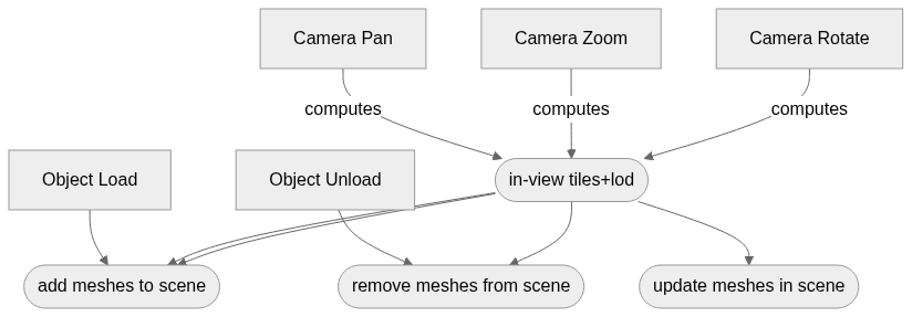
The implementation could have some optimisations done to more correctly identify the in-view tiles, for now it is good enough as a proof of concept, and importantly it is fast. These updates need to happen on each change of view. Any camera interaction like panning, zooming, rotating will need to compute the in-view tiles and update the scene accordingly. Loading and unloading objects also need to update the scene, but these actions do not need to compute the viewbox. We want to avoid removing all the meshes and adding them back into the scene. It is costly to do so, but more importantly, there will be a perceptible flash as the mesh is removed then added. As such, these tiling+LOD changes are treated as sets and only meshes which have had a change are touched.
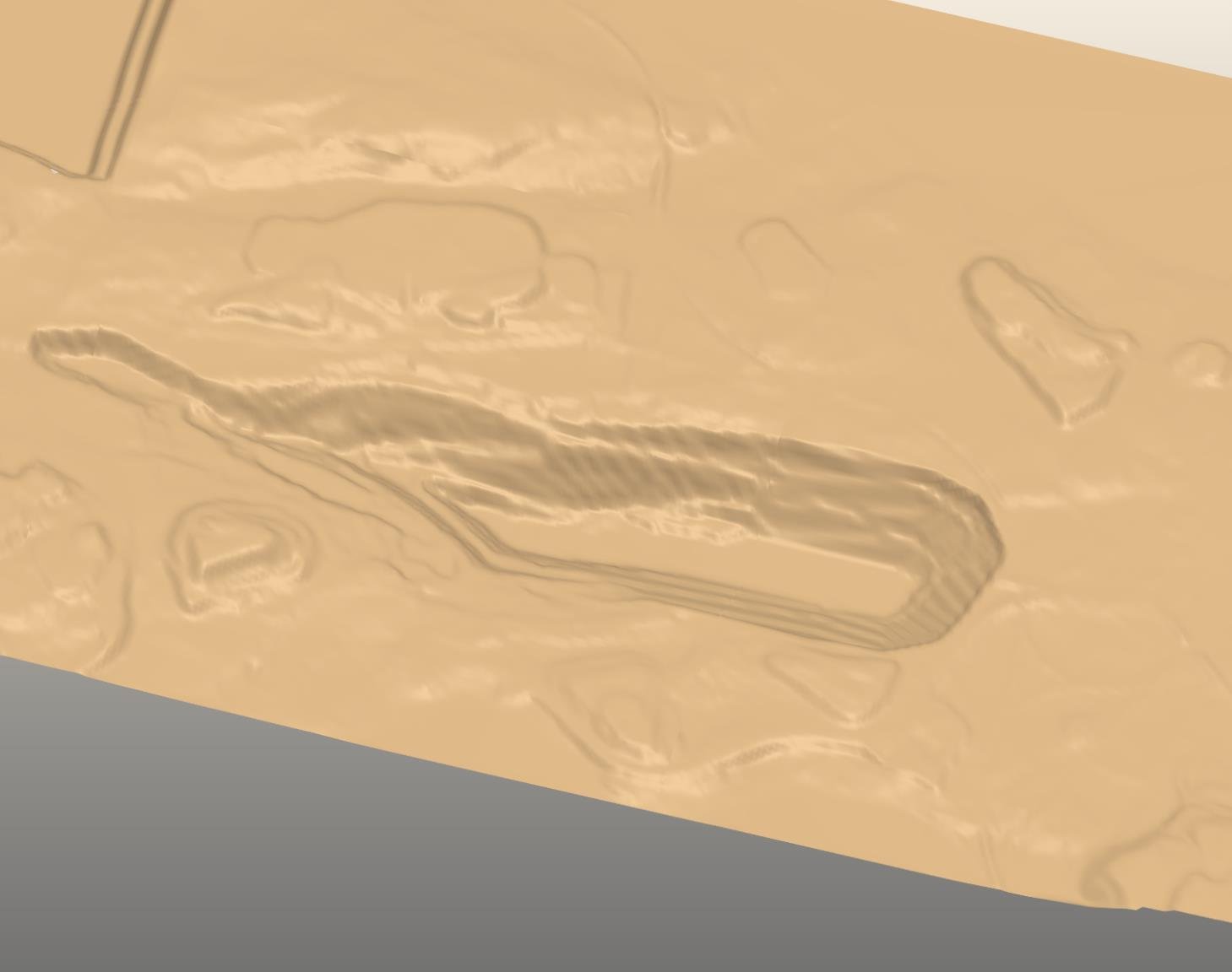
With that, we can visualise a surface!
And does it work?
Yes! Very well! Only including in-view tiles reduces the rendering pressure, and zooming in will swap out the meshes for higher detail ones on the fly. The asynchronous nature of pulling from the store means the meshes will load progressively, which actually has a nice 'loading' effect and provides a similar feeling one gets from mapping software utilising tiling.
However there was a major performance niggle which prompted a structural change. It came down to the loading of tiles at low LODs. At the lowest LOD, there is only 25 data points. This is a tiny amount of data, but the rendering pipeline still needed to reach to the store, read in the data, and process it into a triangle mesh. I thought that concurrently loading them might solve the issue, but the sunk cost of accessing the database stacks up. In testing I had around 450 tiles for a surface, and each tile would take around 1-3ms to read in from the database and load into the scene as a triangle mesh. This adds up, and even working concurrently, it could still take a few seconds to load all the tiles in. One of the issues is that renders would occur within this, which could take a millisecond or so, but it delays fetching the next tile. So tiles would load in progressively but it would feel slow, despite loading the lowest level of detail. When zooming in and the number of in-view tiles reduced, this effect does not happen even though we a now loading in tiles which far greater counts in data points. After a bit of profiling/timing/head banging, it was decided to switch up the tiling paradigm.
Tiles with fixed number of points
So our bottleneck seems to be in accessing IndexedDB for the many in-view tiles. It is worth gathering some data on access times. Each LOD tile consists of a sequence of 4 byte floats (Float32Array) stored as an ArrayBuffer blob. At the lowest LOD resolution of 50m, there would be $(200 / 50 + 1)^2 \times 4 = 100$ bytes of data. At the highest LOD resolution of 0.5m, there would be $(200 / 0.5 + 1)^2 \times 4 = 643,204$ bytes of data. Running through 100-1,000,000 bytes gives average access time tabled below.
| stored bytes | average load time (ms) |
|---|---|
| 100 | 0.5 |
| 500 | 0.7 |
| 1,000 | 0.6 |
| 5,000 | 0.5 |
| 10,000 | 0.4 |
| 50,000 | 1.5 |
| 100,000 | 1.3 |
| 500,000 | 2.5 |
| 1,000,000 | 6.2 |
Here's the data plotted.
So it looks like there is a baseline access time, it is not until around 50 KB of data does the loading of this data start impacting load times. What we want to leverage is a reduction in the number of tiles needing loading, which means larger tile areas, and it looks like even with large tiles we can get away with the speedy load times. Another way to think about this is, if we can reduce the number of tiles to load from 400 to 40, and the individual load times only increase from 2-3ms to 5-6ms, we should see a speed up of 6x.
We can achieve this by fixing the tile grid count, rather than the tile size. Choosing a grid count is somewhat arbitrary, a trade-off between load times and rendering burden. From the previous attempt, a count of 201 at 1m LOD resolution rendered fine, but 0.5m LOD (401 count) started to have stuttering. The count also affects how much coverage a single tile will have. The table below covers using a grid count of 251 vs 101 with various LODs, and how large a coverage the tile would have (this is all talking in one side length). It is worth noting that with a grid count of 251, the LOD data would consume 252,004 bytes, whilst a grid count of 101 would consume 40,804. It is also worth noting that with a grid count of 251, the coverage becomes vast and somewhat defeats the purpose of the tiling at the lowest level of detail. For this attempt, a grid count of 128 is chosen (a nice binary number), from 0.5m to 32m LODs.
| LOD resolution | count | size |
|---|---|---|
| 0.5m | 250 | 125m |
| 1m | 250 | 250m |
| 2m | 250 | 500m |
| 4m | 250 | 1,000m |
| 8m | 250 | 2,000m |
| 16m | 250 | 4,000m |
| 32m | 250 | 8,000m |
| 0.5m | 100 | 50m |
| 1m | 100 | 100m |
| 2m | 100 | 200m |
| 4m | 100 | 400m |
| 8m | 100 | 800m |
| 16m | 100 | 1,600m |
| 32m | 100 | 3,200m |
But fixed counts will not tessellate?
No, they do not, but we can make them neatly nest. There is a reason the LOD resolution in the previous table are in powers of 2, as a LOD becomes more detailed, we can replace one tile with four more detailed tiles. This is a quadtree structure. Quadtrees are great because we can describe hierarchy within the structure, and quickly drill down to detail by bounding child nodes to four quadrants.
It is also easy to identify a node. Since each node will have four children, each child can be assigned a number between 0-3. In binary we need 2 bits to describe all the child locations. I like to use the bits to describe x/y movements, so that the first bit describes the x quadrant, and the second bit describes the y.
bit pattern location 00 bottom-left 01 top-left 10 bottom-right 11 top-right
---------
| 01 | 11 |
|---------|
| 00 | 10 |
 ---------
So we can describe a node in that lives in the top-left corner of the bottom-right parent node with the bit path10_01. In a usual quadtree design the root node would encompass the whole data extents. I will tweak this to use a tessellating grid of the lowest LOD detail (32m) where each cell would be a root quadtree. To identify a tile, the root index in the grid and the quadtree path is used. To go from 32m to 0.5m LODs, we need 6 path elements to reach the highest detail depth. That is $6 * 2 = 12 bits$, so a 16 bit integer will suffice. Another neat property that drops out of the path is the LOD information. If there is no path, this represents the lowest level of detail, a path of 2 bits gives us LOD index 1, 4 bits is index 2, and so on. This saves some indirection on the storage side, we can refer to both LOD and tile ID using a single value.
A bit path can also be decomposed given a leaf's index in terms of x/y numbers. Going down 6 levels results in 7 LODs (including the root) which gives 128 cells (note: this is serendipitous with the 128 grid count size chosen before, this is purely because of the depth of the tree). If for example an index into the 128x128 grid is given such where x = 14 and y = 31, these indices can be decomposed into the leaf's path of 00_01_11_11_11_01 (bottom-left➡top-left➡top-right➡top-right➡top-right➡top-left). The neat thing about the x/y indices is that they each encode the path along their dimension. Take a look at the number 14 in 6 bits of binary: 001110, and 31: 011111. Notice how when interleaved we get the path as before.
x = 14 : 0 0 1 1 1 0
y = 31 :  0 1 1 1 1 1
merge => 000111111101
00_01_11_11_11_01
This is a variant of Morton encoding, and we can use it to generate the leaf tiles that overlap a 2D AABB quickly. If we know the leaf tiles, we trivially know the parent tiles as well!
With this tiling method we will have to rework the whole pipeline; sampling, store loading, viewbox, and mesh creation. We can start at the viewbox, since this will drive the mesh updates. Like before, the viewport is projected onto the world extents in render space, giving an AABB of in-view area. The LOD resolution is also the same calculation. The difference is now the AABB does not bound the tile x/y indices, instead each tile will need to recursively check for intersection to reach the depth. While this sounds more complex, it is quite easy to implement given we are working with AABB extents (intersection testing is easy), and we know the depth we need to reach given the resolution. It can be implemented as a stack to avoid recursing, and the implementation ends up using less code. The number of intersection tests that occur should roughly be constant, either we are very zoomed out which means there will be many tiles but a shallow depth, or there will be few tiles which go deep.
impl ViewableTiles {
    /// Calculate the tiles/lods in view and store them internally.
    pub fn update(&mut self, viewbox: &Viewbox) {
        let world = &self.extents;
        let scaler = world.max_dim();

        // LOD resolution
        // world area
        let area = viewbox.render_area * scaler * scaler;
        // console::debug_1(&format!("area {area:.0} | ha {:.0}", area / 10_000.0).into());
        let lod_res = (area / 10_000.0).powf(0.5) / 2.0;
        let lod_depth = choose_lod_depth(lod_res) as u8;

        let extents = Extents2::from_iter(
            viewbox
                .min_ps
                .into_iter()
                .chain(viewbox.max_ps)
                .map(|p| p.scale(scaler).add(world.origin.into())),
        );

        let mut stack = TileId::roots(world);
        self.in_view.clear();
        self.out_view.clear();

        while let Some(t) = stack.pop() {
            let ints = t.extents(world).intersects(extents);
            let at_depth = t.lod_lvl() == lod_depth;

            if ints && at_depth {
                // simply push this tile into view
                self.in_view.push(t.as_num());
            } else if ints {
                // push the child nodes onto the stack
                stack.extend(t.children());
            } else {
                // does not intersect, we add as an out of view
                // note that this would be at the lowest LOD without overlap of inview
                self.out_view.push(t.as_num());
            }
        }
    }
}
Following the viewbox, the mesh updater needs to handle this new method of tiling. The previous updater was efficient, reusing meshes and storing the backup variant. It was designed to control the layers automatically, and as such was structured around the tiles. The new method is more nuanced, with child meshes needing to be created and disposed of. The method of keeping the lowest LOD around for fast loading is also preferable. It is complicated by the fact that I do not want to create a quadtree in Javascript, as it will be slow/error prone to implement walking through the tree. We can leverage the tile ID in a similar fashion to the previous implementation, where the ID will be mapped to an array of mesh objects that control the rendered mesh. This has the benefit of being flat, but suffers from no good way to 'overwrite' meshes, avoiding mesh creation (which, admittedly, is fast, but it would be preferable to have long-lived meshes). We also want the updating to not stutter or flash. This is tricky, since it means the updating needs to add the new tiles first, then remove the old tiles (in-view), and then populate the out-of-view tiles with the lowest LODs.

The tiles updating can be thought of as 3 sets:
- The original or old rendered tiles
- The new in-view tiles
- The new out-view tiles
Where these sets overlap, there is no change necessary. The first sequence is to load the new in-view tiles. These will overlap with currently rendered tiles (marked 'remove'). Then the old tiles can be removed. Finally, we load out-of-view tiles to provide some data outside the viewbox.
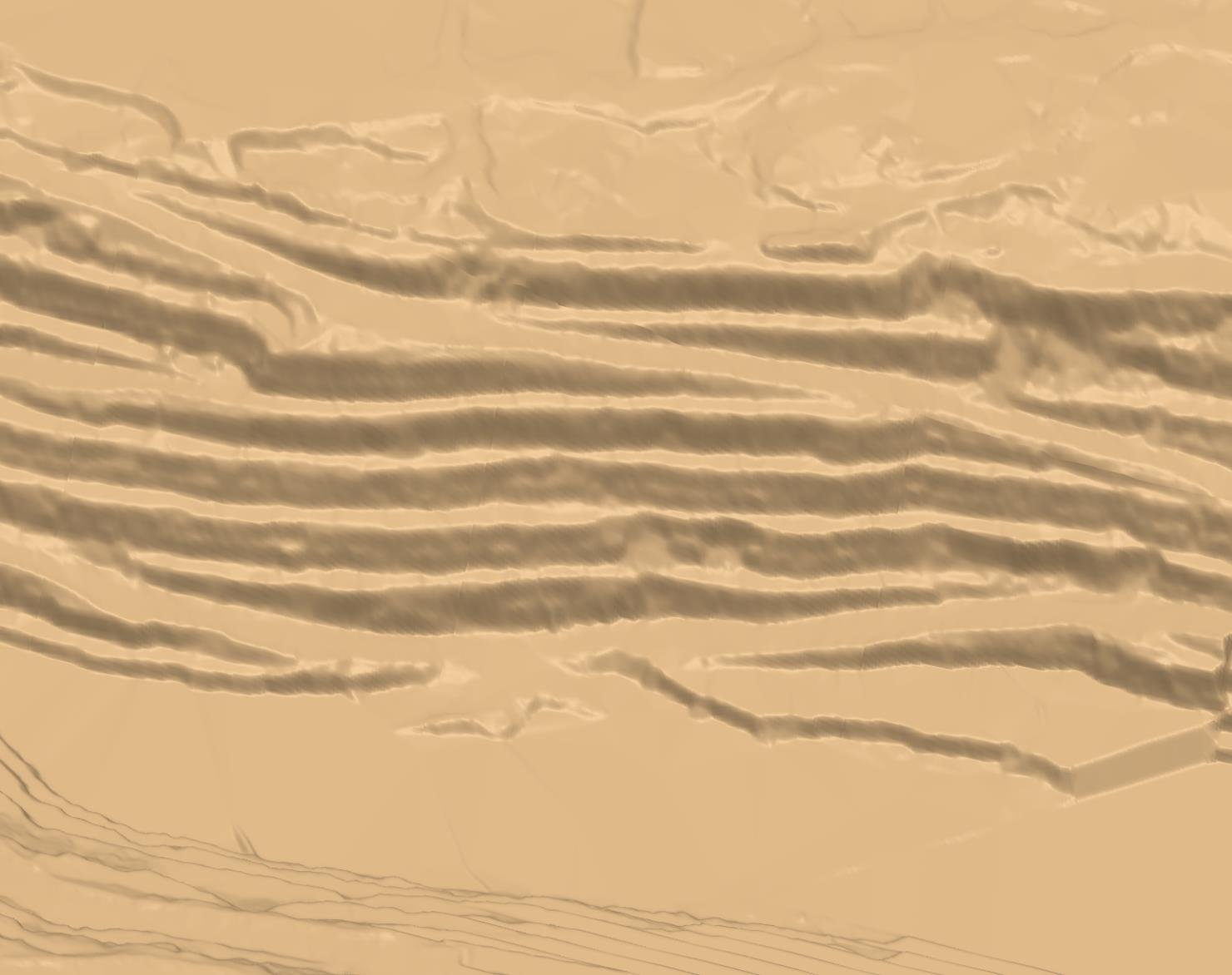
And does that work?
Yep! Not only does it solve the 'slow' loading at low LODs, it also cleans up the implementation that the mesh loading had to go through, reducing indirection through the use of a bit path. Here's some footage of the dynamic loading.
The project is still very experimental, however it shows how structuring a rendering pipeline to utilise tiling and LODs as a first class mechanism will have immediate benefits, despite the additional contextual burden it places on the developer. I am going to extend these mechanisms to other objects (line work, point clouds, etc) to continue to showcase the technology. I would appreciate support! If you have an interest in 3D rendering, you can find the project hosted on Github and open a PR!